Harald Vöhringer, PhD

The Fourier transform has always been somewhat elusive to me. How is it possible to take any kind of sinusoidal signal and decompose it into its constituent frequencies ? I always felt that I lack a deeper understanding and so I recently started to dig into the topic a bit more deeply. Here, I will summarise what I have learned about the discrete Fourier transform by deconstructing its formula step by step.

The discrete Fourier transform

Let's start with the formula itself. The discrete Fourier transform $\hat{U}(f)$ of some input signal $u(t)$ can be written as

where $N$ is the total number of time steps of the signal. Note that $\hat{U}(f)$ is unlike $u(t)$ not a function of time but rather a function of some "test" frequency $f$.

To motivate our discussion, let's consider a concrete example. Say that we are given simple sinusoidal input signal with a frequency of $f=4$ Hz, i.e.

import matplotlib.pyplot as plt
import matplotlib.cm as cm
import numpy as np
import seaborn as sns
f = 4
T = 1
N = 1000
t = np.linspace(0, T, N)
u = np.cos(2*np.pi * f * t) + 1

plt.plot(t, u)
ax = plt.gca()
ax.set(ylabel='Intensity ($u(t)$)', xlabel='Time ($t$)', title='Input signal')
sns.despine(ax=ax)
plt.show()

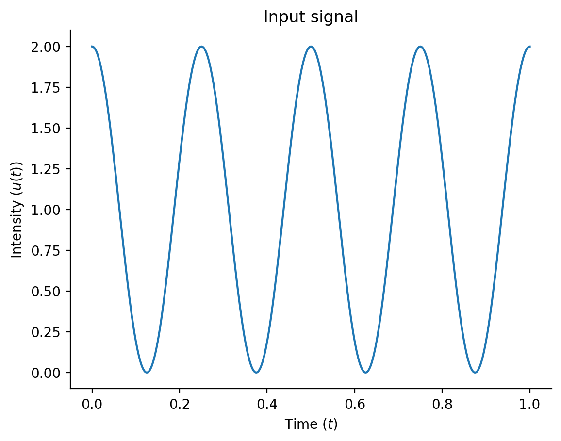
How does the discrete Fourier enable us to extract the periodicity of this signal ?

The exponential term $e^{-i 2\pi ft}$

Let's start by looking closer at the exponential in the formula. Recall that the $e^{it}$ describes the counter-clockwise rotation of a unit vector in the [[complex plane]]. For example, when $t = \pi$ the vector has travelled 180 degrees and when $t=2\pi$ it has reached 360 degrees.

cm = plt.get_cmap('Blues')
t = np.linspace(0, 2 * np.pi, 1000)
r = np.exp(-1j * t)

fig = plt.figure()
ax = plt.gca()

im = ax.scatter(np.real(r), np.imag(r), s=1, cmap=cm, c=t)
cartesian_axis(ax, xmin=-1, xmax=1, ymin=-1, ymax=1, xlabel='Re', ylabel='Im', fontsize=10)
fig.colorbar(im, label='t')

plt.tight_layout()
plt.show()

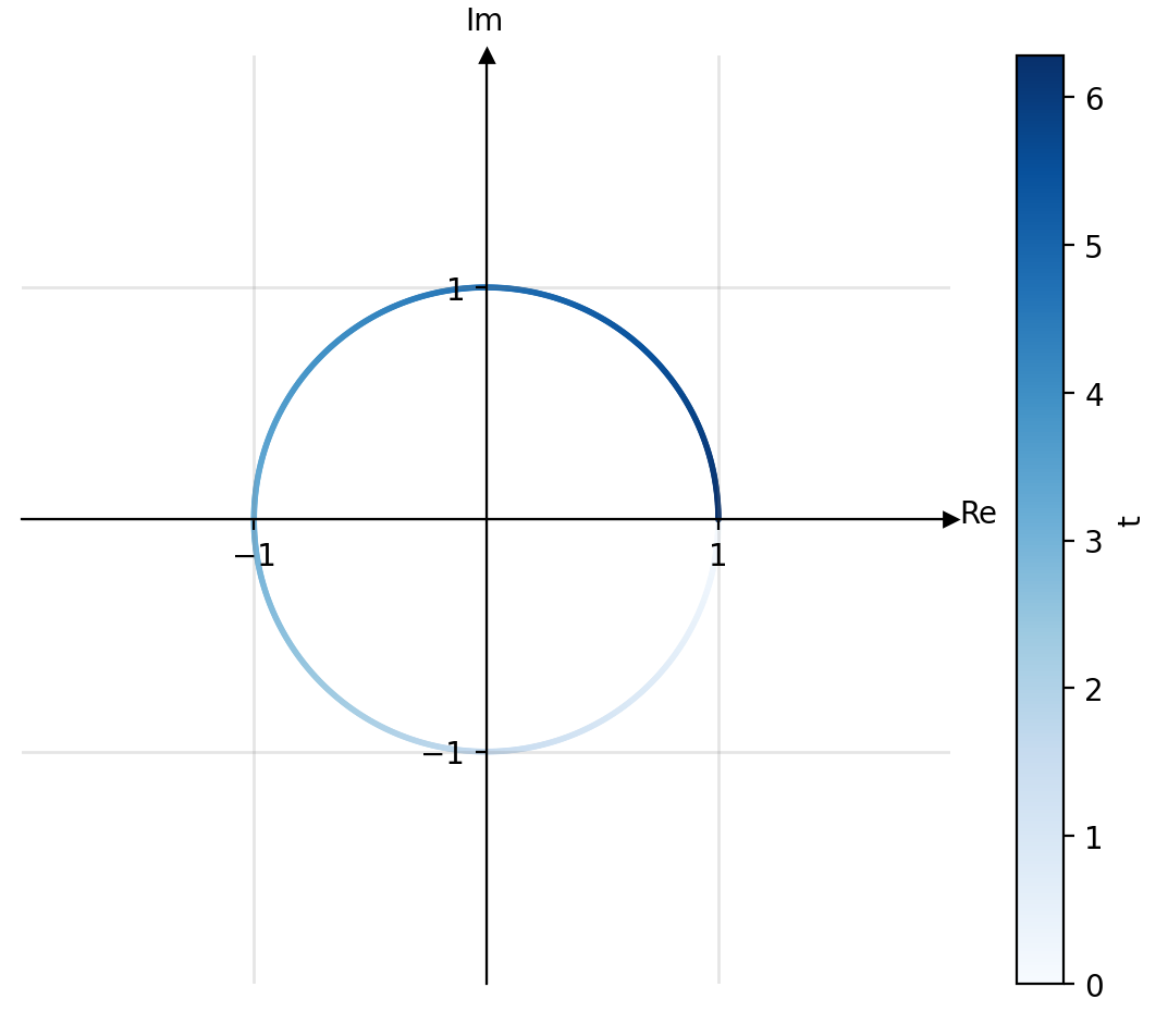
With this in mind it is easy to see what $-i2 \pi f t$ does. First, the minus sign causes the unit vector to rotate into the clockwise direction. In the case of the discrete Fourier transform this happens to be purely a convention. Second, recall that $f=\frac{1}{T}$ where $T$ is the period of the test frequency. So intuitively the term $2\pi f= \frac{2\pi}{T}$ can be understood as the velocity with which we rotate our unit vector in the complex plane. For example, if we consider a frequency of $f=4$ Hz, i.e. we observe 4 cycles per second, then we have $2\pi ft=2\pi 4t=8\pi t$ and see that at $t=1$ we travelled $8\pi$ or 4 full 360 degree rotations.

Multiplying the input signal with the exponential

Let us now now consider both the input signal and the exponential term $u(t)e^{-i 2\pi ft}$ . We start by obtaining a visual intuition by plotting $u(t)e^{-i 2\pi ft}$ for different test frequencies $f\in\{1,\dots,10\}$ Hz.

f = np.arange(1, 10).reshape(-1,1)
t = np.linspace(0, T, N)
u = np.cos(2*np.pi * 4 * t) + 1
h = u * np.exp(-1j * 2 * np.pi * f * t)

fig, axes = plt.subplots(3, 3, figsize=(6, 6))

for i, ax in enumerate(axes.flatten()):
	im = ax.scatter(np.real(h[i]), np.imag(h[i]), s=1, cmap=cm, c=t)
	cartesian_axis(ax, xmin=-1, xmax=1, ymin=-1, ymax=1, xlabel='Re', ylabel='Im', fontsize=10)
	ax.text(.9, 1.7, f"$f=${i+1} Hz")

plt.tight_layout()
plt.show()

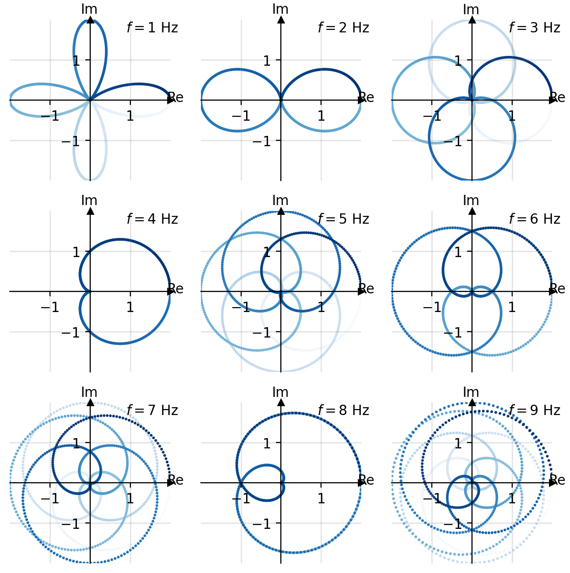
At first sight these graph look quite interesting, don't they. What has happened here ?

The explanation is quite simple. These graphs result from rotating the unit vector with different velocities (i.e. frequencies) and scaling it's length at each time point $t$ with the input signal $u(t)$. In other words, we "wrapped the input signal around a unit circle". Now we have almost everything that we need to understand the formula from above.

Averaging $u(t)e^{-i 2\pi f t}$

So far we have seen that multiplying the input signal $u(t)$ with the exponential term $e^{-i 2\pi ft}$ leads to interesting patterns when the resulting complex numbers are visualised in the complex plane. In the next step, we have to take these values and average them. We can visualise this again on the complex plane by taking the average of the real and imaginary parts of $u(t)e^{-i2\pi ft }$ .

fig, axes = plt.subplots(3, 3, figsize=(6, 6))

for i, ax in enumerate(axes.flatten()):
	im = ax.scatter(np.real(h[i]), np.imag(h[i]), s=1, cmap=cm, c=t)
	ax.scatter(np.mean(np.real(h[i])), np.mean(np.imag(h[i])), color='C3')
	cartesian_axis(ax, xmin=-1, xmax=1, ymin=-1, ymax=1, xlabel='Re', ylabel='Im', fontsize=10)
	ax.text(.9, 1.7, f"$f=${i+1} Hz")

plt.tight_layout()
plt.show()

We can see that the average value stays for most test frequencies around the origin. The only exception is $f=4$ where the right dot shifts for the first time to the right. This shouldn't be too surprising. Recall that we have generated the input signal $u(t)$ using this frequency.

Let's take a closer look at these average values by plotting them onto the complex plane. In the following plot we can track the average real and imaginary parts as a function of the test frequency (shown as the color gradient).

f = np.linspace(1, 6, 1000).reshape(-1, 1)
u = np.cos(2*np.pi * 4 * t) + 1
h = u * np.exp(-1j * 2 * np.pi * f * t)

fig = plt.figure()
ax = plt.gca()
im = ax.scatter(np.mean(np.real(h), axis=1), np.mean(np.imag(h), axis=1), s=1, c=f, cmap='Reds')
cartesian_axis(ax, xmin=-0., xmax=0., ymin=-0., ymax=0., xlabel='Re', ylabel='Im', fontsize=10, )
fig.colorbar(im, label='Frequency $f$')
plt.tight_layout()
plt.show()

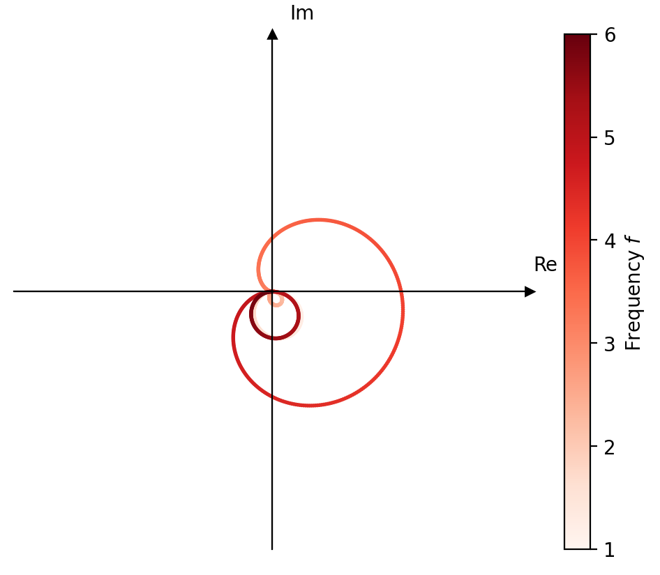
A problem with this representation is that it is quite difficult grasp the relationship with the frequency. For this reason we will simplify things and plot the test frequency against the real part of $\hat{U}(n)$.

plt.plot(f.squeeze(), np.mean(np.real(h), axis=1))
ax = plt.gca()
ax.set(xlabel='Frequency ($f$)', ylabel='$Re[\hat{U}(f)]$')
ax.axhline(0, color='k', ls='--')
sns.despine(ax=ax)
plt.show()

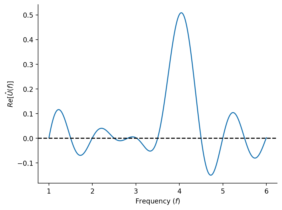
From this plot it becomes very evident with which frequency we created our signal at the first place. In summary, we have seen that performing a discrete Fourier transform encompasses "wrapping" the input signal around a oscillating unit vector (with different speeds) in the complex plane. When the test frequency matches the frequencies underlying the input signal, we observe shifts average real parts of these trajectories, enabling us to identify important frequencies.